Tutorial: First project
This is a simple example for making analysis files for OpenFOAM with XSim.
Analysis summary
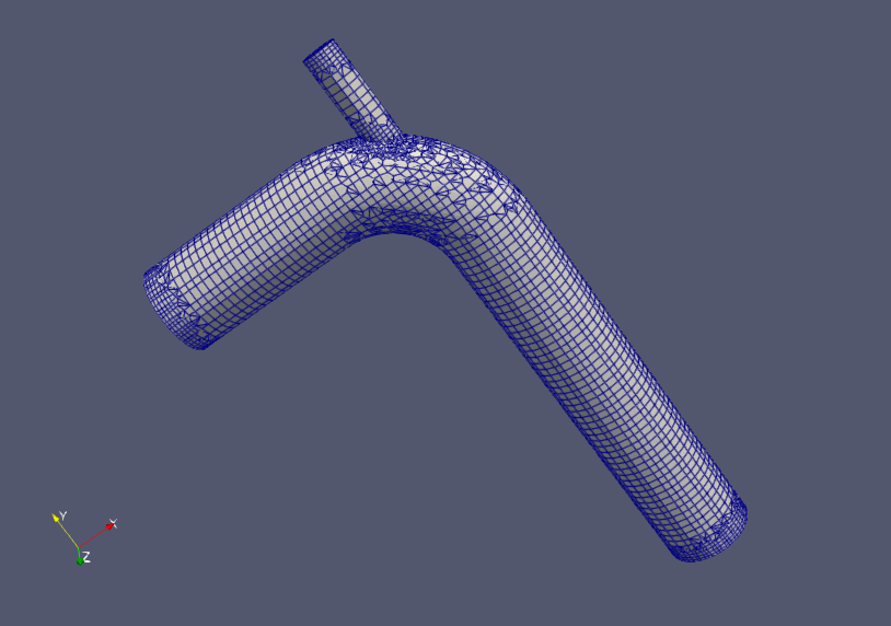
In this tutorial, we will configure an analysis of pipes internal flow. The bending pipe flow and narrow straight pipe flow will join together into one flow in the analysis.

Creating an analysis configuration file
-
Prepareing shapes and Starting XSim
Download zipped sample STL files from "tutorial-pipes.zip" and extract it. Then start XSim with following button.
-
Crateing a project
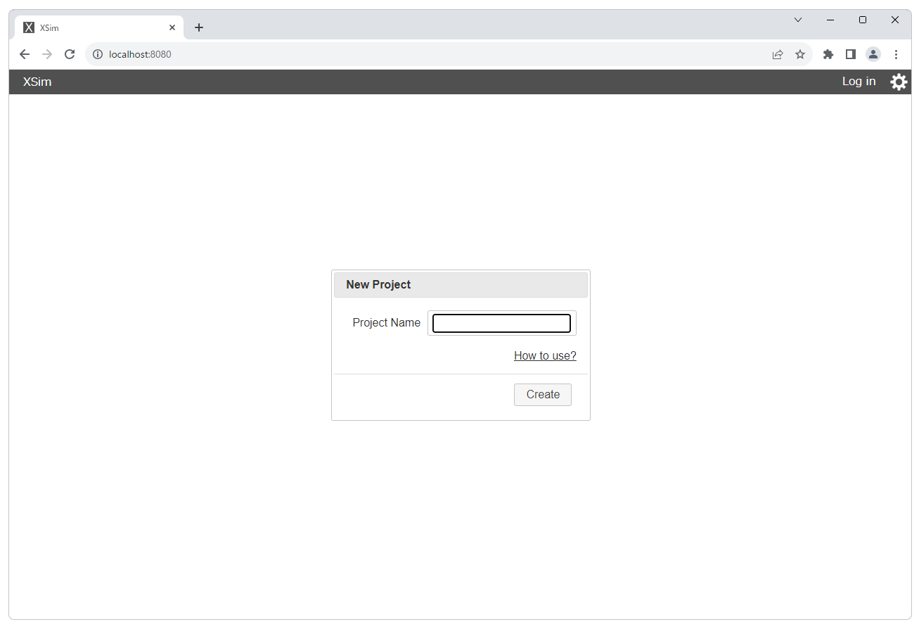
Type "MyFirstProject" as Project Name and click button to create project.
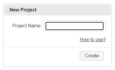
-
Features of each view
XSim has 3 views. "Navigation view" (left side), "Control view" (center), and "3D view" (right side).
If you click the item like "Mesh" and "Basic Settings" in Navigation view after loading model shapes, a corresponding setting page will be displayed in Control view. And you can also confirm model shapes in 3D view.
If you want to change language settings, click
button at top-right of window to show preference dialog. Current version of XSim supported "English" and "Japanese".
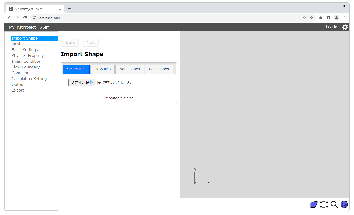
-
Import Shape
To begin with, import shapes from the downloaded STL files.
Drag&Drop the STL files "Inlet1.stl", "Inlet2.stl", "Outlet.stl" and "Wall.stl" onto the area below "Drop files" tab. So the STL files will be loaded and the shapes will be displayed in 3D view.
3D view operations with mouse is following.
3D view operations Rotation Zoom Pan Mouse left button + Drag Mouse wheel roation Mouse middle button + Drag You can confirm each region by clicking region name in Navigation view. The selected region is filled with orange in 3D view. To deselect region, click region name agein.
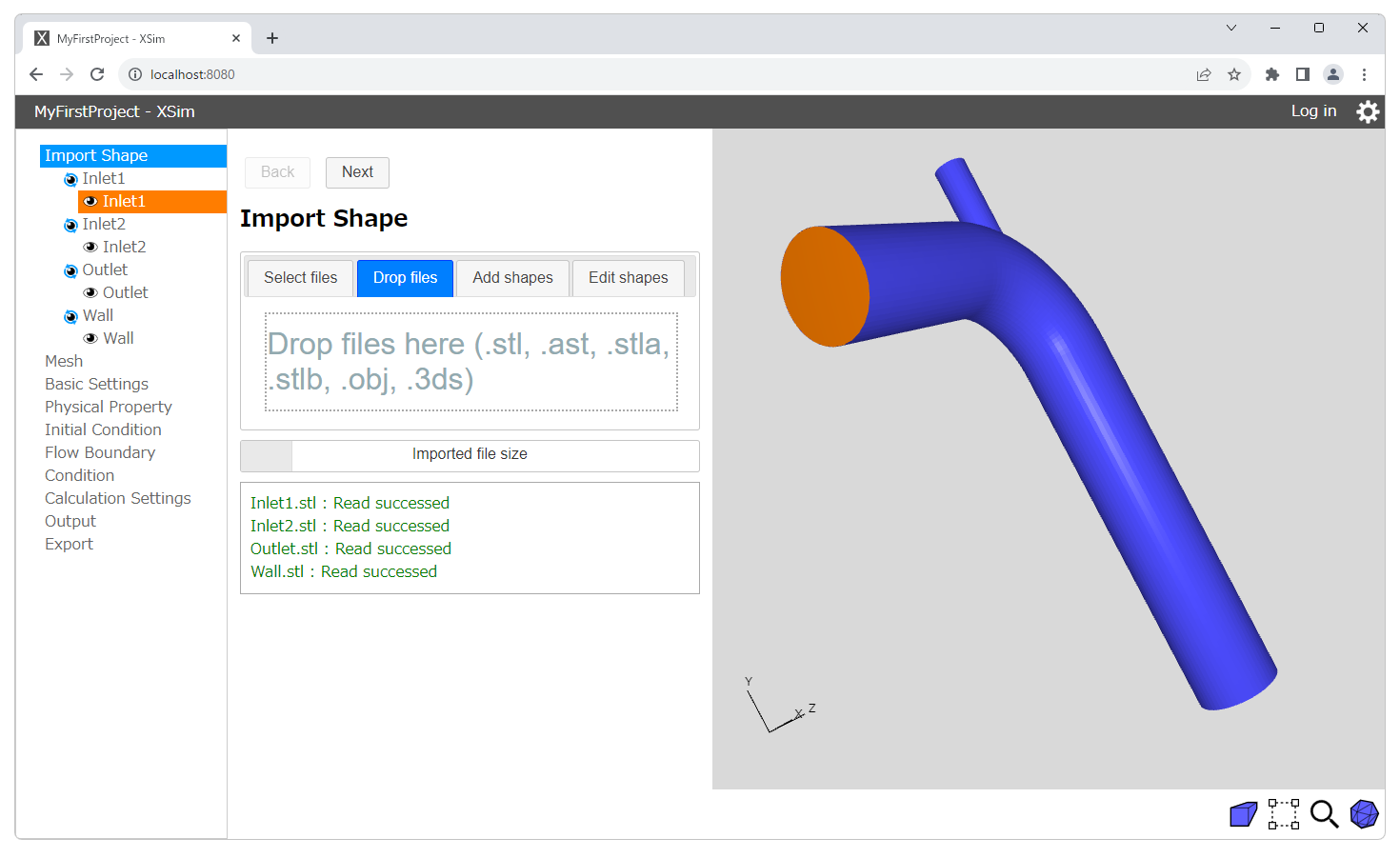
Loading the STL files and select region "Inlet1". Click button to go to Mesh settings page.
-
Mesh
In Mesh settings page, a base mesh area and a coordinate that defines computational domain will be displayed with white line in 3D view.
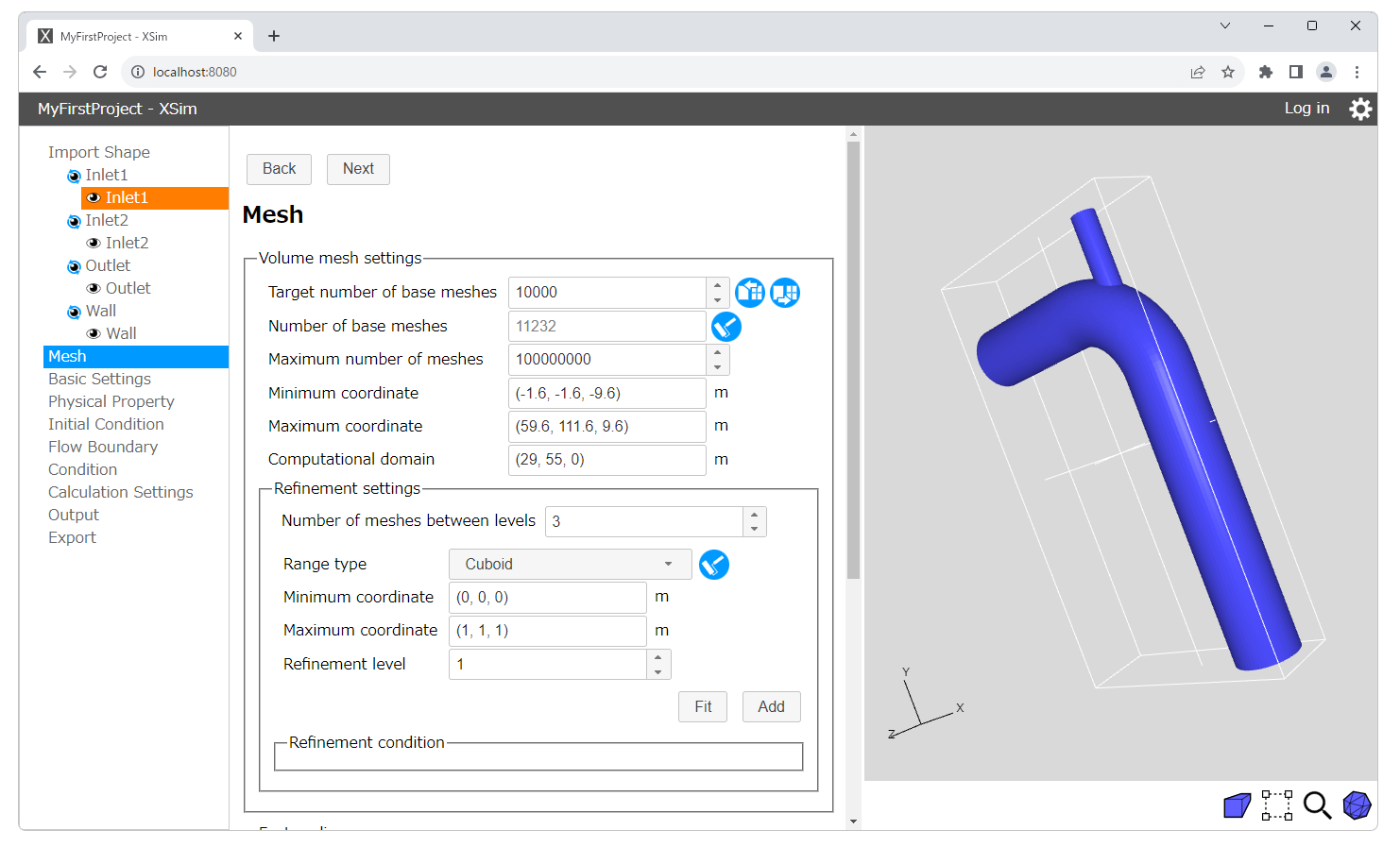
Click "Target number of base meshes" input-box and set the value to "50000".
Click "Computational domain" input-box and set the coordinate to (50, 55, 0).
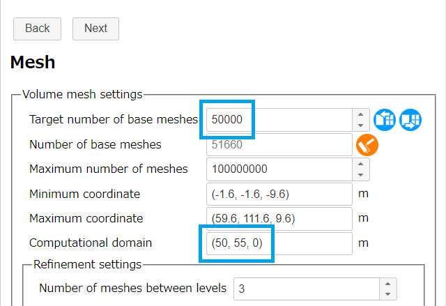
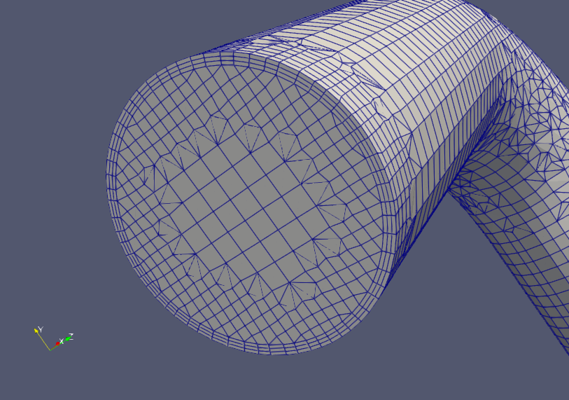
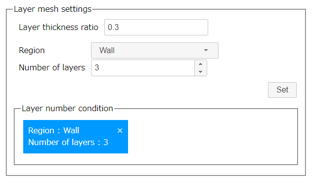
Next, we will set layer mesh settings. Select "Wall" as region from a combobox in "Laye mesh settings" and set "Number of layer" to "3".
Then click button. When the settings are done properly, blue rectangular block will be displayed.
When you want to delete and reset the settings, click "×" button at top-right of a block.
Click button to go to Basic settings page.
-
Basic settings
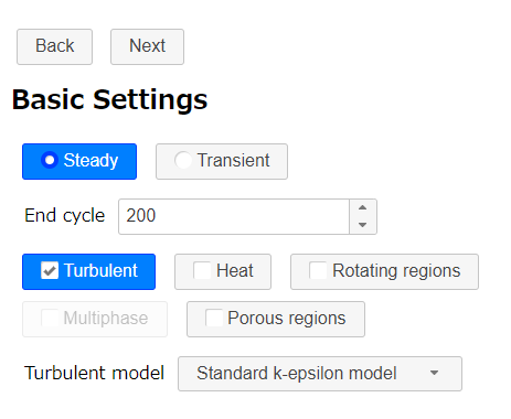
In this tutorial, we will execute steady analysis until 200 cycles and use standard k-epsilon model as RANS model.
So It is not necessary to change a settings in this page. Leave the settings as default.
Click button to go to Physical Property page.
-
Physical Property
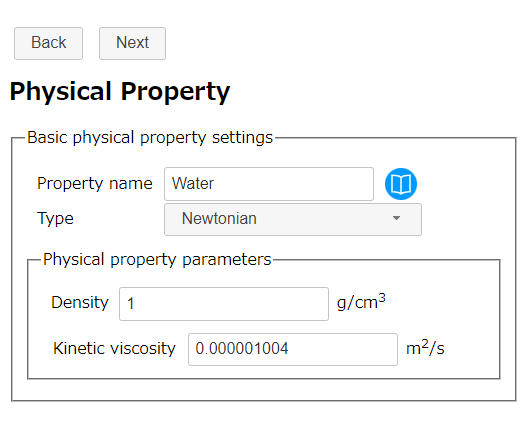
In this tutorial, we will use water as fluid.
So It is not necessary to change a settings in this page. Leave the settings as default.
Click button to go to Initial Condition page.
-
Initial Condition
In this tutorial, we not need to edit this settings.
Click button to go to Flow Boundary Condition page.
-
Flow Boundary Condition
In this page, we set flow bondary condition for the analysis.
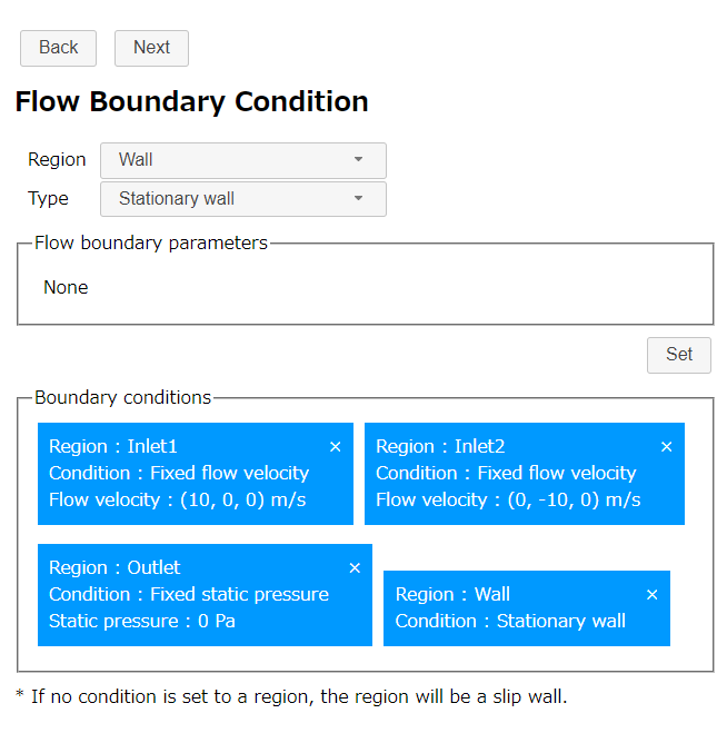
At first, select "Inlet1" as region and "Fixed flow velocity" as type from comboboxes. Then change "Flow velocity" value in "Flow boundary parameters" to (10, 0, 0) m/s and click button to set the boundary condition to the region.
In the same way, set "Fixed flow velocity" (0, -10, 0) m/s to region "Inlet2".
Next, select "Outlet" as region and "Fixed static pressure" as type from comboboxes. After confirming the "Static pressure" value is set to "0" Pa, click button to set the boundary condition to the region.
At last, select "Wall" as region and "Stationary wall" as type from comboboxes. click button to set the boundary condition to the region.
The conditions will be dislpayed as blue blocks in "Boundary conditions". If you want to delete and reset a settings, click "×" button at top-right of a block.
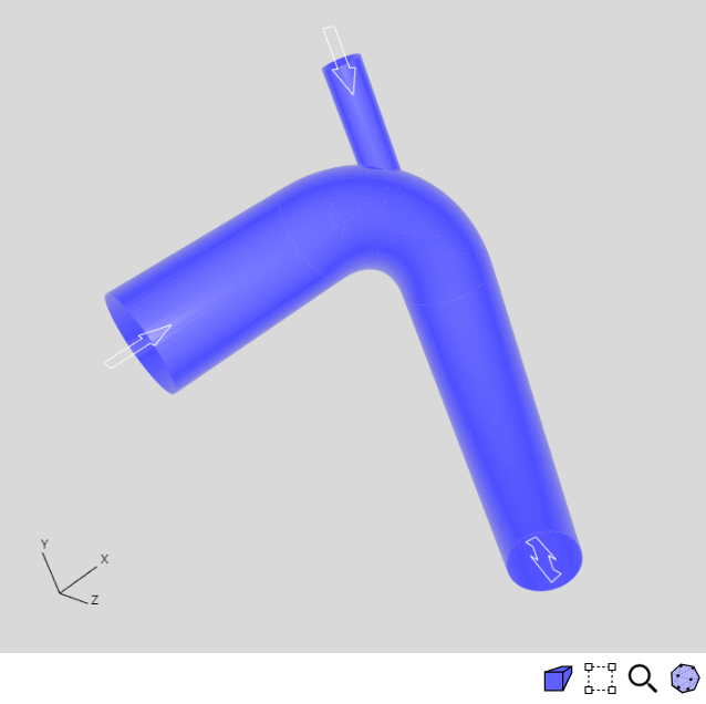
Some types of condition will be displayed as an arrow in 3D view and you can check the region that the condition is applied. Transparency of 3D shapes can be switched with clicking
.
Click button to go to Calculation Settings page.
-
Calculation Settings
In this tutorial, we not need to edit this settings.
Click button to go to Output page.
-
Output
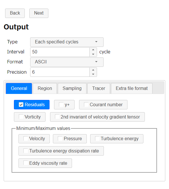
In this page, we can set calculation output settings. Confirm "Type" is set to "Each specified cycles" and change "Interval" to 50 cycle(s).
Click button to go to Export page.
-
Export
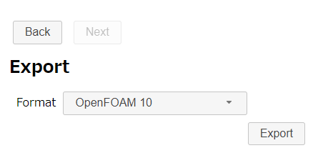
Finally we finished all setings. Click button to export the analysis setting as zipped OpenFOAM case directory "MyFirstProject.zip". The zip file download starts immediately.
You can close XSim on webbrowser. If you are logged in XSim, you can save the created data on the cloud and re-edit it later. We won't save data in this tutorial.
Running a calculation
You need OpenFOAM on your machine. If you have not installed OpenFOAM on your machine, please refer to "OpenFOAM for Windows 10 | OpenFOAM" and install OpenFOAM.
Extract "MyFirstProject.zip". There is a bash-script "Allrun " in the case directory. So run the script to make mesh and calculate the OpenFOAM solver by following command.
If gnuplot has been installed, chart of residuals for monitoring will be displayed in the calculation.
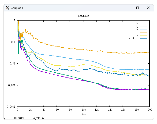
Confirming a calculation result
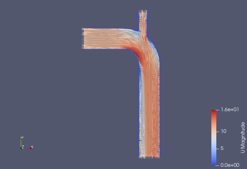
After the calculation finishing, you can check mesh and calculation result with the ParaView. So run ParaView to visulalize the mesh and the result by following command.
Calculating and Visualizing operations are same as standard OpenFOAM operations.
